
Variation in image examples
Having extracted all images, it’s interesting to see the variation in color, lighting, etc. of the material.
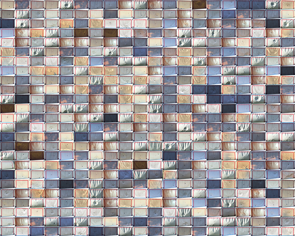
Having extracted all images, it’s interesting to see the variation in color, lighting, etc. of the material.
My initial working assumption was that I could exclude the part of finding the exact location of the goal/canvas in each frame as
Although (1) and (2) still hold, (3) barely even held for indoor sessions where most parameters were fixed for the recording duration and definitely does not hold for uncontrolled outdoor sessions. An underlying idea of using a canvas is to provide something flexible and portable for players, which comes with the side effect of less rigidity. On the other hand, few materials hold up to being hit by a hockey puck in full speed (even expensive match-quality hockey goals become dented) so non-rigid materials and mounting methods is also a way of handling this.
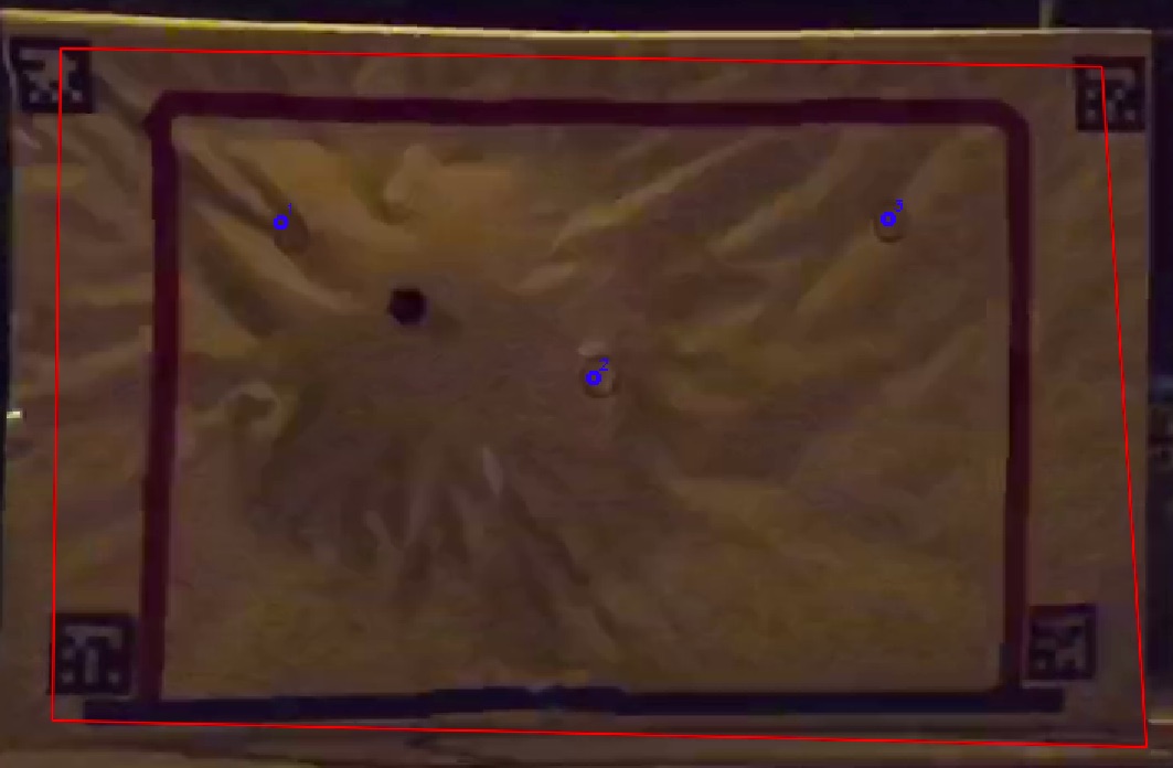
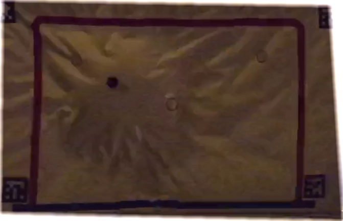
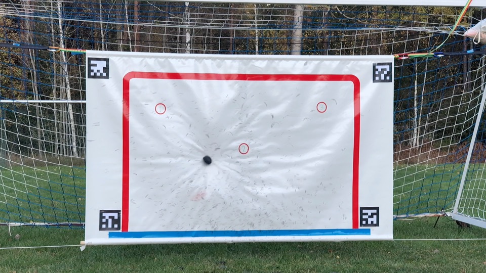
The problem, then, is to find a transformation matrix (a homography) that maps coordinates in the below canvas illustration to coordinates in an actual video frame.

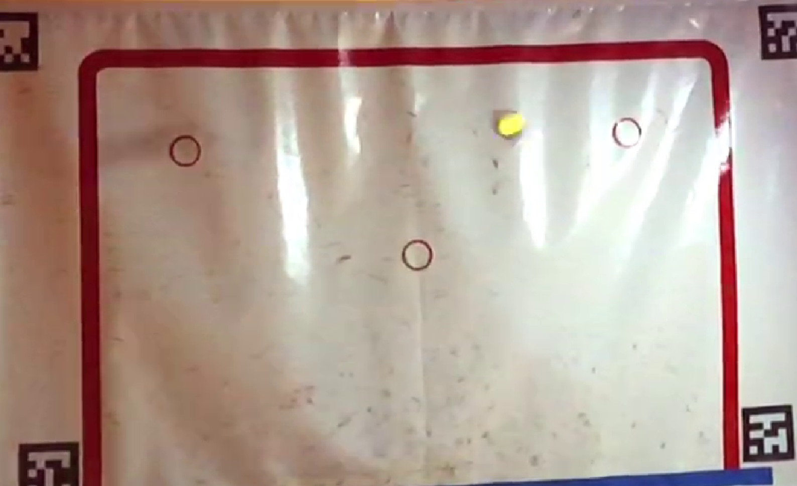
In short, I use SIFT feature detection on both illustration and video frame to find keypoints that can be used to match the two. I then use a brute force matcher to find the set of most similar keypoints, which then is used to construct a matching homography matrix using RANSAC. Then this is used to construct a mask representing the corners of the canvas in order to extract only the part of the canvas representing the goal, with very little background visible.
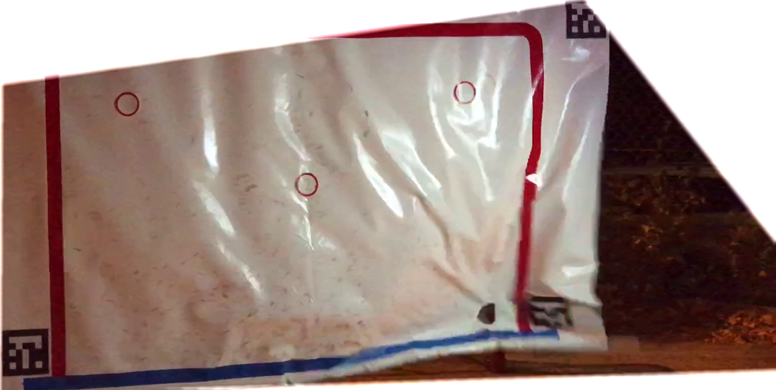
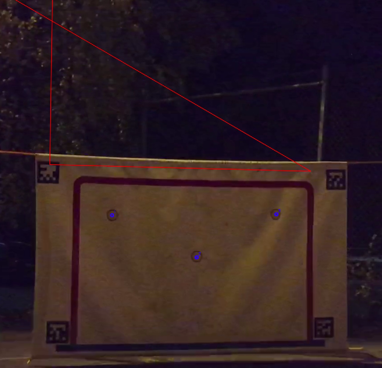
The problem, like so often in computer vision, is that this does not work perfectly every time. A small fraction of the frames (out of thousands) has intermittent homographies suddenly jumping to something like the below (and then back again).
One solution could be to use the average corner coordinates over a number of frames in order to even out the effects of these bad homographies. However, what if one frame was really bad, like shown below? Then instead of having one bad set of corner coordinates, all coordinates based on an average that included the bad frame would be poor.
A better solution seems be to use something like Kalman filtering for each corner, adjusting the parameters so the coordinates would adjust slowly and big jumps would be treated as sensor errors. So I implemented this and let the kalman filtering run for six frames before using the homography to capture any example. I also reset the kalman filter after having processed each shot since the canvas could potentially be repositioned by the player in between each shot.
At first, this appeared to be a working fix but then I noticed that the initial frame was bad for a round (see below). This caused the starting points to be off and even though the Kalman filter slowly adjusted itself to a good representation of the canvas corners, it took much more time than the six frames I had alloted. Why not let it run 60 frames? Because calculating the homography based on SIFT and brute force matching is a choice of precision rather than processing time.
At this point, I adjusted my assumptions and instead of letting every shot being independently analyzed and use the same Kalman filter over the whole round of shots. Doubling the number of prior frames used should be enough to adjust to reasonable changes in positions of tripod and canvas between shots. As long as the first homography in a whole session is okay, the rest should be too.
One might imagine that using more prior shots would be better, right? Not entirely. One of the prior frames resulted in the below homography, from which the kalman filter did not recover during the shot. A very similar problem to the one discussed in relation to using the average over several frames. In some sense this brings the whole problem back to square one.
In the long run, I probably need to experimentally find out what a reasonable homography is. That is, for example, look into the range of plane normals that can be expected given a mobile camera on a tripod, the canvas level and hanging some distance off the ground.
For now, some of the bad cases, like the one above, can be handled by checking that the corners resulting from the transformation are ordered properly (the left corners having smaller x-coordinates than the right corners, etc.) Also the ratio of side lengths should be within some margin. This does not completely fix the problem but results in far fewer erroneous goal corners.
Edit: I also managed to improve things by adjusting the SIFT parameters for the stencil based on it being an illustration. This is also something I need to look into more as it is not obvious what an optimal set of parameters look like for this application. Also, at this moment I can only visually inspect the images – and there are thousands.
Edit 2: The processing time for all session excepth the eleventh took 13 hours and 12 minutes. The result was 3441 examples of the puck just having hit the canvas and 3519 examples of the canvas not yet having been hit. Based on visual inspection, very few examples are based on a non-optimal homography and none of the examples are invalid. The total, just shy of 7000 examples, should be enough data for now.
There was a little snow in the air so I drove out to the football field, hoping for snow flakes in the recorded videos but no such luck. It is yet another thing I’m hoping the completed model will be invariant to (but that might be pushing it).
In most cases there is an obvious difference between the canvas before having being hit by a puck and after. The question, raised in a previous post, is how to deal with the edge cases.
There are basically five different three-sequence cases, all sharing
not hit.hit class.hit, albeit not necessarily
a good example of a puck just having hit the canvas.hit class based on the similarity
with images of pucks very close to hitting the canvas (the not hit class),hit class.hit class.hit (especially if the puck just grazed the edge of
the canvas).hit (sometimes it does and sometimes
it does not).Avoiding false positives must be the priority since identifying an image as a hit when it is not could result in very bad measurements as the puck could be far from its eventual impact point, perhaps not even visible in the image. Missed identifications are less problematic as there will be a sequence of images showing the puck having hit the canvas and it will be a slow and gradual decrease in accuracy with later frames. Thus, we want to err on the safe side and not include frames if they are not visually distinct enough.
After a puck hits the canvas, with each frame, the movement of the canvas
becomes less and less similar to the movement after first impact. Eventually
it turns into something that bears resemblence to the effects of strong wind.
Thus, we also want to avoid assigning later frames as examples of the class
hit.
Based on the above, a set of tentative rules for assigning classes are:
ambiguous to frames in between clear examples in order to
skip these frames for now,hit so the examples
provide clear examples of the puck just having hit the canvas,Yesterday, I recorded seven rounds in artificial light. This is yet another tricky situation I wanted to capture on video in order to later be able to test for invariance. That a computer vision algorithm can be made invariant to everything it is not supposed to detect or measure is never really the case, especially in non-controlled situations like this.
Artificial light is problematic in several ways. For one, artificial light is generally much more dim that natural light, which is why indoor photographs often turn out blurred. A camera could try to counteract this by increasing the aperture and increasing the sensitivity of the sensor but the latter has the sideeffect of noisy images.
Secondly, artificial light usually causes hard shadows as the amount of ambient light is so low compared to the point-source directed light. Thirdly, the color temperature of artificial light is different from that of natural light. This goes especially for street lighting and other similar sources of light where the light quality is relatively unimportant to energy efficiency.

Last and most problematic, many light sources tend to pulse or flicker. This is not always noticeable by eye but depending on type, these lights are recharged/reignited according to the frequency, or twice the frequency, of the power source. This is a known phenomena and one usually counteracts it by recording in a frequency that divides twice the power source frequency. Sweden has a power grid based on 50 hz and this means that 20 hz, 33.33 or 50 hz is safe to use. One problem here is that at least iPhones only offer multiple of 30 hz (since 60 hz is the power grid frequency in the US, one can assume). So recording in the slo-mo mode and 120 hz causes very noticeable pulsing as can be seen in the video below.
Augmenting the overhead lights with a sidemounted runner’s headlamp seems to have improved the situation but also caused canvas glare (see video below).
Now, the benchmark comparison here is really human analysis of the video material so if it is too dark to record a video, it would make it impossible to accurately analyze and thus makes it out of scope for this study. The accuracy in regards to these recordings definitely dropped because it was dark, primarily because it was difficult to tell the puck from its shadow, but it was by no means too dark.
With that said, from a training perspective, the light required to be able to train is much less than to record the training. An existing training location might thus have to be fitted with additional lights.
